Stitched Value Model for Diffusion Alignment

1ETH Zรผrichยท 2Googleยท 3University of Copenhagen

TL;DR

Make any clean-image reward model work on noisy diffusion latents.

Same reward model — now scoring noisy diffusion latents directly, at the quality you expect on clean images. The first practical recipe.

โ‘กWhat we do

EXISTING clean image โ†’ Reward model โ†’ reward StitchVM small compute OURS noisy latent โ†’ Value model โ†’ reward

StitchVM takes a pretrained pixel reward model and, at small compute cost, lets the same model score the noisy intermediate latents — not just the final clean image.

โ‘ขThe impact

One fix Replace the heavy effort to denoise a noisy latent to calculate a pixel reward โ†’ with a direct StitchVM score. The four wins that fall out โ†“

DPS

3.2× faster

higher quality · โ†“50% GPU memory

FK steering

33% lower cost

via a more efficient scaling axis

DRaFT

+30% GenEval

& 22–26% fewer GPU-hours

DiffusionNFT

55%+ GPU-h saved

2.3× faster training

โ‘   THE QUESTION

Q: Is this noisy latent on its way to a good reward?

Most diffusion alignment methods come down to answering this question along the denoising trajectory.

๐ณt noisy latent we glance at this denoising ๐ณ0 clean latent decode ๐ฑ0 final generation what it will become โœ“ good reward how valuable will it be?

Diffusion sampling will turn the noisy latent $\mathbf z_t$ into a final generation $\mathbf x_0$. Every alignment method has to answer this from a glance at $\mathbf z_t$ alone: how valuable will the final $\mathbf x_0$ be?

Formally, this is the value function $V_t(\mathbf z_t)$ — the expected reward of the clean image $\mathbf z_t$ will eventually denoise to:

$$V_t(\mathbf z_t) \;=\; \mathbb E\!\left[\,r(\mathbf z_0)\,\big|\,\mathbf z_t\right].$$

Across both inference-time and training-time alignment, evaluating $V_t$ is the common need — three examples:

Inference — gradient guidance e.g. DPS
$$u^{r}_t(\mathbf z_t) \;=\; u_t(\mathbf z_t) \;+\; c_t\,\nabla_{\mathbf z_t} V_t(\mathbf z_t).$$
The current velocity $u_t$ at each step is nudged by the value gradient, giving a corrected velocity $u^r_t$ used for sampling.
Inference — particle sampling e.g. FK steering
$$G(\mathbf z_{t_k}, \bar{\mathbf z}_{t_{k-1}}) \;=\; f\!\left(V_t(\bar{\mathbf z}_{t_{k-1}}),\; V_t(\mathbf z_{t_k})\right).$$
At each step, each particle draws a proposal $\bar{\mathbf z}_{t_{k-1}}$ and is reweighted by a potential $G$ — some function $f$ of $V_t$ at the current and proposed states (specific methods choose different $f$). Particles are then resampled in proportion to $G$.
Training — reward-based finetuning e.g. DRaFT, DiffusionNFT
$$\arg\max_{\theta}\; \mathbb E_{\mathbf z_0 \sim p_\theta}\!\left[r(\mathbf z_0)\right] \;-\; D_{\mathrm{KL}}(p_\theta \,\|\, p).$$
Each training iteration evaluates $V_t(\mathbf z_\tau)$ at an intermediate noisy $\mathbf z_\tau$ in place of the terminal reward $r(\mathbf z_0)$ — so the rollout can stop early instead of denoising all the way to a clean image.
โ‘ก  THE PROBLEM

Matching pixel reward quality on noisy latents has been impractical

So methods approximate $V_t$ instead — each approximation with cost and estimation problems.

Learning $V_t$ directly would be the cleanest fix — no bias, no variance, no extra evaluations. But matching a foundation-scale pixel reward model (CLIP, HPSv2, Aesthetic Predictor) on noisy latents has meant training at their scale, redone for every new backbone or reward. So practitioners approximate $V_t$ instead. Two workarounds dominate — each with its own price:

Tweedie approximation
Mechanism: approximate $\mathbb{E}[r(\mathbf{z}_0)\mid\mathbf{z}_t]$ by $r(\hat{\mathbf{z}}_0)$ with $\hat{\mathbf{z}}_0 = \mathbb{E}[\mathbf{z}_0\mid\mathbf{z}_t]$ from one denoiser call (Tweedie).
๐ณt denoiser
$\hat{\mathbf z}_0$
VAE
$\hat{\mathbf x}_0$
reward model rฬ‚ COST denoiser + VAE + reward per call
$V_t(\mathbf{z}_t) \approx r(\mathbb{E}[\mathbf{z}_0 \mid \mathbf{z}_t])$
โš  ISSUE Jensen-gap bias — worst exactly when noise is highest Monte Carlo rollouts used in most RL post-training methods
Mechanism: draw $N$ samples $\mathbf{z}_{0,i} \sim p(\mathbf{z}_0\mid\mathbf{z}_t)$ via full rollouts, average $r(\mathbf{z}_{0,i})$. Unbiased, but variance $\propto 1/N$.
๐ณt denoise ร— T steps denoise ร— T steps denoise ร— T steps VAE ร— N reward model ร— N average rฬ„ COST N full denoising rollouts per call
$V_t(\mathbf{z}_t) \approx \tfrac{1}{N}\sum_{i=1}^{N} r(\mathbf{z}_{0,i}),\ \ \mathbf{z}_{0,i} \sim p(\mathbf{z}_0 \mid \mathbf{z}_t)$
โš  ISSUE high variance at small N — full rollouts make large N expensive โœ“ ADVANTAGE no bias, no variance, no decoder — what StitchVM unlocks Direct learning of Vt THE IDEAL TARGET
Mechanism: train a model $V_t$ directly on noisy latents to predict the true expected reward $\mathbb{E}[r(\mathbf{z}_0)\mid\mathbf{z}_t]$.
Vt learned directly rฬ‚ one forward pass. no decoder. no rollouts.

Practitioners settle for the red rows above because matching pixel-reward quality on noisy latents has meant retraining at foundation scale. StitchVM avoids that: it transfers, instead of retraining.

โ‘ข  THE UNLOCK

๐Ÿง‘โ€๐Ÿคโ€๐Ÿง‘ Pixel-reward quality.
On noisy latents.
Via model stitching.

At the cost of a short finetunenot retraining anything from scratch.

Why this works: at the right depth, the internal features of a pretrained diffusion model are almost linearly compatible with those of a pretrained pixel reward model. So we keep the head of the diffusion model frozen (already native to noisy latents), keep the tail of the reward model (it already produces the score), and join them with a small stitching layer — initialised by a closed-form linear fit, then briefly finetuned together with the reward tail on unlabeled images. The stitched model inherits the reward model's predictive skill, but now operates directly on noisy latents.

PRETRAINED Diffusion backbone ๐ณt  (noisy latent) layer 1 layer iโ˜… โœ‚ CUT layer N (drop) KEEP THE HEAD PRETRAINED Pixel reward model ๐ฑ0  (clean image) layer 1 (drop) โœ‚ CUT layer jโ˜… layer M (reward) KEEP THE TAIL STITCHED ๐Ÿง‘โ€๐Ÿคโ€๐Ÿง‘ StitchVM ๐ณt  (noisy latent) diff layer 1 diff layer iโ˜… โ‡„ stitching layer reward layer jโ˜… rฬ‚ noisy-latent Vt ONE FORWARD PASS

The result is a noisy-latent value model at pixel-reward quality, built in hours on a single GPU — no training from scratch, just a transfer.

โ‘ฃ  THE REACH  ·  WHY IT MATTERS

One $V_t$. Every alignment recipe.

Build $V_t$ once. Drop it into every alignment recipe — inference-time guidance, particle sampling, training-time finetuning — and watch each one get cheaper at the same time.

Cheaper. Sharper. Less biased.

DPS gradient guidance

DPS steers denoising along $\nabla V_t$ — the gradient is the guidance signal
$u^{r}_t(\mathbf{z}_t) \;=\; u_t(\mathbf{z}_t) \;+\; c\,\nabla V_t(\mathbf{z}_t)$
quality & speed of $\nabla V_t$ matter — computed at every denoising step
STANDARD (TWEEDIE) long backprop ยท biased gradient ๐ณt denoiser
$\hat{\mathbf z}_0$
VAE ๐’Ÿ
$\hat{\mathbf x}_0$
reward ๐‘Ÿ rฬ‚
$\nabla_{\mathbf z_t} \hat r$ via backprop · 3 networks differentiated
+ Jensen-gap bias: Tweedie sets $V_t(\mathbf{z}_t) \approx r(\mathcal{D}(\text{denoiser}(\mathbf{z}_t)))$, not the true $\mathbb{E}[r(\mathbf{z}_0)\mid\mathbf{z}_t]$.
low ฯƒ high ฯƒ bias worst at high noise — exactly where DPS guidance works hardest WITH STITCHVM NEW direct gradient ยท exact ๐ณt
$V_t$
noisy latent in ยท scalar out
$V_t(\mathbf{z}_t)$
$\nabla_{\mathbf z_t} V_t$ via 1 backward ยท no decoder ยท no Tweedie
Mechanism: $V_t$ takes the noisy latent $\mathbf{z}_t$ directly, so $\nabla_{\mathbf z_t} V_t$ is one autograd call through $V_t$ — no decoder differentiation, no denoiser differentiation, no Tweedie approximation. Faster AND less biased at every step.

FK steering particle sampling

STANDARD FK STEERING scale axis โ†‘ N ยท add particles ๐ณ1 denoiser + VAE + reward w1 ๐ณ2 denoiser + VAE + reward w2 ๐ณ3 denoiser + VAE + reward w3 โ‹ฎ โ‹ฎ โ‹ฎ ๐ณN denoiser + VAE + reward wN RESAMPLE over N particles โ‹ฎ next N
FK steering's scaling axis is $N$ — each particle needs one denoiser + VAE + reward call to compute its weight, so cost $\propto N$.
ZOOM IN ON ONE PARTICLE WITH STITCHVM NEW scale axis โ†‘ M ยท per particle ๐ณt one of N
$\times M$ draws
$M$ next-step candidates
$\mathbf{z}^m_{t-1} \!\sim p(\mathbf{z}_{t-1}|\mathbf{z}_t)$
$V_t$
cheap ยท $M$ evals
scores noisy latents
score 1 โ˜… best score 3 score M argmax COST PER +1 ON EACH AXIS +1 N denoiser + VAE + reward +1 M
$V_t$
no extra denoiser call · no VAE
StitchVM opens a cheap axis — many $M$ evals cost less than one expensive N-particle.

Supervised at every noise level.

DRaFT · AlignProp · DiffusionNFT direct reward finetuning · RL post-training

STANDARD rollout cost: T steps ยท supervision only at ๐ณโ‚€ ๐ณ1 ๐ณ0 r
$T$ denoiser calls per iteration
gradient flows back through all $T$ denoiser calls
Supervision gap: reward is defined on the clean image $\mathbf z_0$ — intermediate noisy latents $\mathbf z_t$ get no direct learning signal (high-noise steps remain dark).
WITH STITCHVM NEW rollout cost: ฯ„ steps ยท supervised at every ฯ„ ๐ณ1 ๐ณฯ„
$V_t(\mathbf z_\tau)$
only $\tau$ denoiser calls ($\tau \!\ll\! T$)
substitutes terminal reward
gradient through only $\tau$ denoiser calls — no full unroll
Supervision at every noise level: $V_t$ scores noisy latents directly, so $\tau$ can be picked anywhere on the trajectory — high-noise steps finally get signal.
WHERE THE LEARNING SIGNAL LIVES
STANDARD
only at $\mathbf{z}_0$
STITCHVM
signal at every $\tau$
incl. high ฯƒ
high ฯƒ (noisy) ฯƒ โ†’ 0 (clean)
$V_t$ lights up the whole trajectory — high-noise steps that were dark now learn.

โ‘ค  THE WINS  ·  RESULTS

Drop-in for every recipe.
Quality up, cost down.

The same StitchVM — one noisy-latent $V_t$, built once by stitching — plugged into four very different alignment methods. Across DPS, FK steering, DRaFT, and DiffusionNFT it delivers better quality with materially lower compute.

DPS ยท gradient guidance

3.2× faster

higher quality on nearly every reward×metric pair ยท โ†“50% peak GPU memory

FK steering ยท particle sampling

33% lower cost

via a more efficient scaling axis — $(N{=}8, M{=}6)$ matches standard FKS at $N{=}14$

DRaFT ยท direct reward finetuning

+30% GenEval

higher score across all metrics & 22–26% fewer GPU-hours

DiffusionNFT ยท RL post-training

55%+ GPU-h saved

2.3× faster training, higher scores on every metric

RESULT 1 ยท NOISY-LATENT VALUE MODEL

StitchVM retains the reward model's capability on noisy latents.

Across three diffusion backbones (SD 3.5 Medium/Large, FLUX) and four reward models (OpenAI CLIP, DFN-CLIP, HPSv2, Aesthetic Predictor), StitchVM closely tracks the original clean reward model at low noise and degrades gracefully as noise rises — substantially beating both VAE-stitching and NoisyCLIP retraining at LAION-400M scale. The expensive "train a noisy-latent reward from scratch" baseline is no longer needed.

Zero-shot image-text retrieval (Avg. Recall@1) on MSCOCO and Flickr30K, vs. noise level ฯƒ
Preference accuracy on HPDv2 and ImageReward benchmarks, vs. noise level ฯƒ Aesthetic SRCC on AVA test split, vs. noise level ฯƒ Legend: clean reward, NoisyCLIP, VAE-stitching baselines, and StitchVM variants

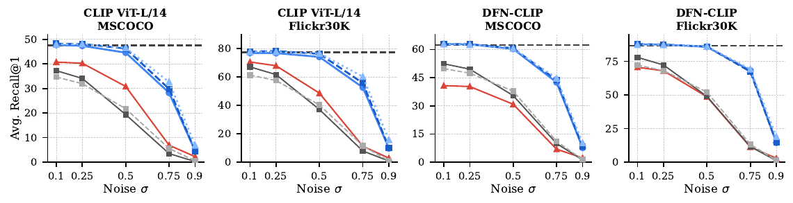
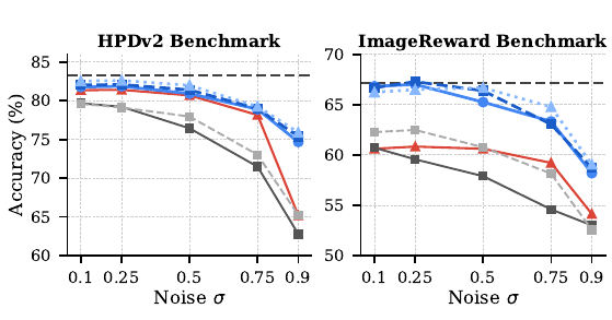
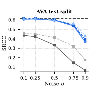
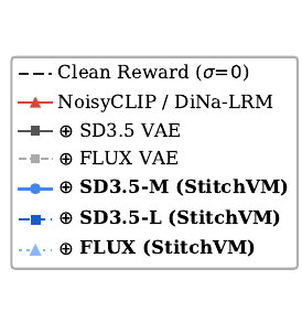
Results of StitchVM on latents with different noise levels. $\oplus$ denotes stitching of a reward model with a pretrained diffusion module (VAE encoder or DiT). StitchVM (blue) tracks the clean reward (dashed line) far better than VAE-stitching or NoisyCLIP, across retrieval, preference, and aesthetic benchmarks.

RESULT 2 ยท A NEW SCALING AXIS FOR FK STEERING

Scaling along $M$ beats scaling along $N$.

Cheap $V_t$ scoring unlocks a second scaling axis on FK steering: instead of adding more particles ($N$), each particle spawns $M$ proposals scored by StitchVM at near-zero marginal cost (partial-DiT inference + stitching head, shared with the next denoising step). On FLUX with HPSv2 reward, FK steering + StitchVM at $(N{=}8, M{=}6)$ matches standard FKS at $N{=}14$ with 33% less compute, and is strictly above the $N$-only curve everywhere.

HPSv2 score vs GPU-hours on FLUX, comparing N-scaling (FKS) against (N,M)-scaling (FKS+StitchVM)

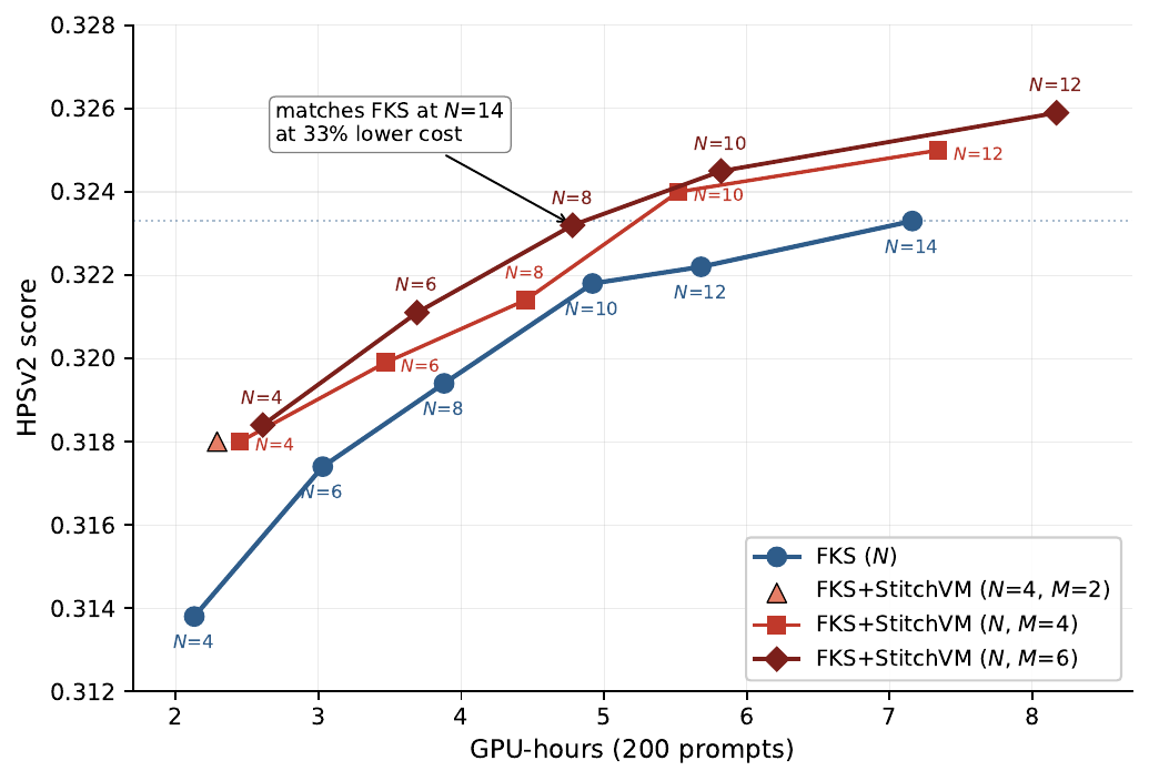
HPSv2 score vs. GPU-hours on FLUX. Blue: standard FK steering scaling $N$. Red/dark-red: FK steering + StitchVM scaling $M$ at fixed $N$. The StitchVM curves dominate the standard one across the whole compute range.

RESULT 3 ยท TRAINING-TIME ALIGNMENT

Same target, $\tau/T$ the rollout cost — better quality on top.

On SD 3.5 Medium at $512{\times}512$ with DFN-CLIP and HPSv2 as training rewards, replacing the terminal reward $r(\mathbf z_0)$ with the StitchVM value $V_t(\mathbf z_\tau)$ (early-stop at intermediate $\tau$) cuts wall-clock training cost dramatically and raises every metric:

  • DRaFT: 22โ€“26% fewer GPU-hours, plus higher quality — StitchVM provides direct $V_t$ supervision at intermediate noisy latents, including high-noise regions where standard DRaFT had to truncate backprop.
  • DiffusionNFT: 55%+ fewer GPU-hours while reaching higher GenEval / ImageReward / PickScore / HPSv2 / DFN-CLIP scores.
GenEval vs GPU-hours: DRaFT-1 and DRaFT-3, with and without StitchVM
DRaFT · direct reward finetuning
GenEval vs GPU-hours: DiffusionNFT vs. DiffusionNFT + StitchVM
DiffusionNFT · RL post-training

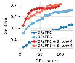
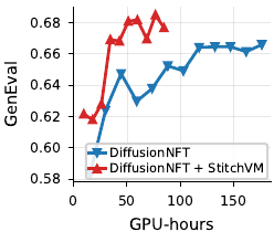
GenEval vs. GPU-hours on SD 3.5 Medium with DFN-CLIP + HPSv2 reward. Red: with StitchVM. Blue: baseline. Adding StitchVM matches the baseline at roughly half the GPU-hours and keeps climbing past it.

Each StitchVM itself is a one-time, lightweight build: $\approx$ 10 GPU-hours at $512{\times}512$ (24โ€“32 GPU-h at $1024{\times}1024$) on GH200 — trivial relative to the savings it enables downstream.

Citation

@article{go2026stitchvm,
    title   = {Stitched Value Model for Diffusion Alignment},
    author  = {Go, Hyojun and Chung, Hyungjin and Truong, Prune and Bhat, Goutam
               and Mi, Li and An, Zhaochong and Zhao, Zixiang and Narnhofer, Dominik
               and Belongie, Serge and Tombari, Federico and Schindler, Konrad},
    journal = {arXiv preprint arXiv:2605.19804},
    year    = {2026}
}